Newton's Law of Cooling

WEBBOT
NAMES, STATION AND PERIOD

Newton's Law of Cooling

I. DATA COLLECTION

1. Open PSLexcelerator and SELECT the TEMPERATURE probe icon and CALIBRATE by typing in the number taped to your temperature probe for PROBE A and by choosing extended. Say YES to placing it in the column to the right of $C:$C. Next, Click on the EXPERIMENT CLOCK in column C and tell the probe to collect 3 samples per second for 5 minutes producing a total of 900 samples. Next go over to PSL on the menu and click on PREVIEW MEASUREMENTS to make sure that your PSL interface is working. When the temperature stabilizes, note and record this initial temperature as your original ROOM TEMPERATURE value for use in your spreadsheet later. ________________

2. After the ROOM TEMPERATURE appears to be stable, get a sample of hot water and place the probe into the water. While still in PREVIEW, watch the probe's temperature increase until it seems to stabilize at a temperature in the range between 80 -100^oC. When this occurs, leave the probe in the water, STOP PREVIEW, go over to PSL on the menu and click on FAST DISPLAY, CREATE FAST GRAPH. After the graph appears on your screen, click on the green "G" icon to start recording your measurements. The PSL will begin to record the probe's temperature data on your graph. After about 3 -5 seconds, take the probe from the hot water and hold it VERY STILL in a "draft free" location until it cools back down to room temperature OR until the time runs out.

3. When the computer is finished taking data, move to FILE, SAVE AS, and save your file with the following filename format: period_station_temp. Record your filename here ________________

[For example, a student in 3rd period at lab station #6 would save his file as period3station6temp [NOTE that you should NOT add a file extension -- PSL automatically adds a .xls extension while saving.]

The PSL program will then let you input a description. Be sure to include your names and the date in the description. Don't forget to unplug the PSL adapter from the AC outlet at your table.

4. After you have saved your file, EXPERIMENT (CLOCK) TIME should be in column C and (PROBE A) TEMPERATURE in column D. In cell E5 type A-RT; in cell E6 type C; in cell F5 type LN(A-RT); in cell G5 type Room; and in cell G6 enter just the numerical value (do not include °C) of the original room temperature recorded in step 1 above.

5. You are now going to program the cells in column E so that the room temperature value in G6 is subtracted from every value recorded under Temp A by the PSL probe - this will calculate the probe's relative temperature, that is, how much higher the probe's temperature was above room temperature.

First go to cell E7 and type =D7-$G$6 and press ENTER. To highlight column C, keep your cursor in E7, press SHIFT (keep it engaged) and use the DOWN ARROW to highlight as much of column E until you reach the last row where column D has an entry. Then release the SHIFT key, and press ALT Edit, Fill Down. This will copy your formula throughout column E. When this has been successfully accomplished, update your file by clicking File Save. You can also drag your mouse down column E, but be careful to start in E7 and to not overshoot your last entry (somewhere around E907).

6. Now go to cell F7, type in the formula =LN(E7) and press ENTER. Format this cell entry by going to FORMAT, CELLS, NUMBER, 3 decimal places. This formula also needs to be filled down throughout all of column F. Do this by first placing the cursor on F7, and then pressing SHIFT and the DOWN ARROW simultaneously. When you reach the last row where column D has an entry, release the SHIFT key, and press ALT Edit, Fill down. This will copy your formula throughout column F. You can also drag your mouse down column F, but be careful to start in F7 and to not overshoot your last entry (somewhere around F907).

7. While at the bottom of column F, look over the last entries in both columns E and F. Since the natural logarithm function is only defined on domain values for x > 0, make sure no entries in column E are 0 or negative; if they are, they should be accompanied by ERROR or #NUM statements in column F. Those data points must be deleted from your columns before you create your next graph in step 9. You can remove them by placing your cursor in each BAD cell and pressing the grey DELETE key.

8. Resave your file. [File Save]

9. We are now going to create and EXCEL graph (called a CHART) from the data recorded in columns C and F. Begin by placing your cursor in C7, hold down the SHIFT key and DOWN ARROW simultaneously until you have highlighted all entries in column C. Then, CAREFULLY press down the CTRL key and release the SHIFT key. Do NOT release the CTRL key! Column C should remain highlighted. While continuing to keep the CTRL key engaged, use the mouse to move your cursor to F7, press down the SHIFT key (CRTL is still engaged!) and highlight column F as well. When both columns are highlighted, release both the SHIFT and CTRL keys and move over on the menu to INSERT, CHART. Choose xy-scatter, type in the title as your lab station number and group members' last names, x-axis is time (sec) and y-axis is LN (A - RT). Turn off LEGEND. Finally choose SAVE AS NEW SHEET. Your graph (CHART1) should now appear on its own worksheet. Check it for any mistakes, and if everything is okay, print it by moving to ALT File, Print. To correct an error, just click on that region of the graph and you should get an active window for editing.

10. Resave your file. [File Save]

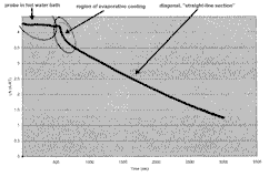
11. Click on your GRAPH, a + should appear on your graph telling you the co-ordinates of any given data point. Drag the cursor along the graph until you reach what appears to be the beginning of the longest, diagonal "straight line section" of the graph (do not choose the flat plateau that initially starts your graph, that region represents the time when the probe was in the hot water bath.).

Record the time of that initial location here ____________.

13. We must now determine the equation of the straight line segment's regression line. This is done by clicking on the graph to get the yellow squares n , then move to chart on the menu, add trendline, linear, and under Options, choose display equation and R² values on chart. When this is complete, print (ALT File Print) your graph and resave your file. [File Save]

14. Mathematically, the half-life represents the amount of time required for a given quantity to be cut "in half." Our probe's data for relative temperature (A-RT) vs time displays the behavior of an exponential decay. It is therefore a reasonable next step to determine the probe's half-life.

At this time, we will calculate the half-life of your group's PSL temperature probe by using the following equation and the slope from your graph of LN(A-RT) vs time:

form field

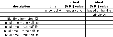
15. In EXCEL, open your spreadsheet and fill out the following data table by scrolling down your data table in column A until you find the time you recorded from step 12. Note the corresponding value for A-RT in column C and record it in your chart. Then scroll down to the time closest to the next time calculated in your chart in step 15 and record that time's corresponding value for A-RT in your chart. Continue this procedure until all 180 seconds have been examined. Then complete the column entitled ideal (A-RT) value.

form field

II CONCLUSION

Did the amount of heat radiated by the probe, as reflected by the changes in its relative temperature [A-RT] in Step 15, behave according to the definition of half-life? Why or Why not? Support your answer by using you data analytically to calculate a percent difference/error for your closest example.

form field

________________________________________________________________________

EXTRA CREDIT: Explain and give a specific procedure for each of the following spreadsheeting terms, operations and skills:

INSERT A CHART (13 x 2) WITH FORM - blanks to be filled in

saving a file with a new name _____

saving a file while keeping its current name _____

opening an existing file _____

cell address _____

fixing the number of decimals in a number _____

centering an entry in a cell_____

notation which begins EVERY formula _____

notation to raise a number to a power_____

notation to add up the entries from C1 to C10 _____

notation to take the square root of the number in cell D2 _____

notation to take the natural logarithm of the number in cell D2 _____

coping a formula in a topmost cell throughout a column__________________________________

freezing the cell address A5 in a formula so that it will not change when the formula is copied elsewhere ________